Introduction

One of the most important steps in developing a model for machine learning is tuning hyperparameters to ensure it generalises to unseen data. A model that fits the training set well but performs poorly on anything else is useless, so care should be taken in ensuring that in-sample performance characteristics of a model are representative of real world performance also. The most simple of these methods is of course using a holdout set, which allows for an easy way to estimate performance on out-sample data but when used as part of the model iteration process, is usually is also overfit to some degree.

The next iteration on this idea is using $k$-fold cross-validation. We split the training data set \((X, y)\) into \(k\) disjoint subsets \((X^{(1)}, y^{(1)}), (X^{(2)}, y^{(2)}), \ldots, (X^{(k)}, y^{(k)})\), and then loop \(k\) times, each time using one of the \(k\) subsets as a holdout set and training on the remaining \(k-1\) subsets. We then are left with \(k\) test scores, which are commonly summarised by their median or mean.

Often one run of cross-validation is completed and we compare the mean score with that from a baseline model. In this article we will explore an extension of this moving from comparison of two point estimates of performance to using T-tests to quantify how statistically significant the improvement is. Testing hypotheses about the relative performance of different parameterisations of the same model allows us to also tune hyperparameters using the same ideas.

Using $k$-fold cross-validation

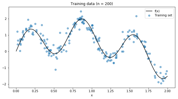
Let’s use a simple example to demonstrate these techniques. We will use numpy to generate a simple non-linear function that we try to fit for the rest of this article.

TRAIN_SIZE = 100
TEST_SIZE  = 1000
SEED = 1
NOISE_VAR = 0.25

def f(X):
    y = np.sin(4*X)
    return y.reshape(-1, 1)

def add_noise(y):
    return y + np.random.normal(0, NOISE_VAR, size=y.shape[0]).reshape(-1, 1)

def generate_training_data(size):
    return np.sort(np.random.rand(size)*2).reshape(-1, 1)

X_train = generate_training_data(TRAIN_SIZE)
y_train = add_noise(f(X_train))

X_test = generate_training_data(TEST_SIZE)
y_test = add_noise(f(X_test))

Now we will use a decision tree to try to fit this function. Let’s try all the values for max_depth from 2 to 15, with 5-fold cross-validation to choose the best parameterisation.

tree_params = {'max_depth': range(2, 16)}
k = 5

tree_gs = GridSearchCV(DecisionTreeRegressor(), tree_params,
                       cv=k, scoring='neg_mean_squared_error')

tree_gs.fit(X_train, y_train)

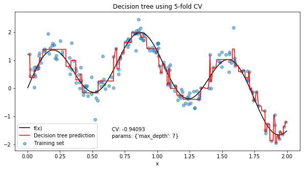
The choice of hyperparameter that give the highest average cross-validation score was a max depth of 7, for an average mean squared error of 0.94093 across the 5 folds. But how good is 0.94093? We can compare it with the other values of max_depth to see how much better the chosen value is, the type of maxima and judge how much changing this hyperparameter actually affects the mean squared error.

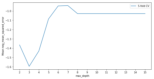
We note here that since scikit-learn always tries to maximise a function, the loss function used here is negative mean squared error.

In this example it looks like the best value for max_depth is somewhere between 6 and 8. Since this is a relatively smooth maxima we may choose to average the predictions from trees with a max depth of 6, 7 and 8. It looks like depths greater than 8 offer no further improvement in fit, so generally we’ll prefer to take less complex models and avoid depths above 8.

Using T-tests

When using $k$-fold cross-validation we get an average over \(k\) scores from different training and test sets. We can think of the average as a draw from some distribution of test scores conditional on the model that we fit to the training data. Among all models we generally want to pick the model that has the distribution of test scores with the highest possible mean. If we assume that the distribution of average test score for a model are normally distributed (by CLT) with some unknown variance, we can use hypothesis testing to compare the draws from different distributions to see if there is a meaningful increase in the performance when moving from one model to another.

Concretely, suppose we have two models \(\mathcal{M}_A\) and \(\mathcal{M}_B\). \(\mathcal{M}_A\) is a model we use as a benchmark and \(\mathcal{M}_B\) is a model we hope outperforms the benchmark. Assume that the average test score for \(\mathcal{M}_A\) and \(\mathcal{M}_B\) are distributed as \(\mathcal{N}(\mu_A, \sigma^2_A)\) and \(\mathcal{N}(\mu_B, \sigma^2_B)\) respectively. Then we are interested in testing the hypotheses

\begin{array}{rcl} H_0 &:& \mu_A \geq \mu_B \\
H_1 &:& \mu_A < \mu_B \\
\end{array}

Testing this hypotheses using the draws collected in from repeated iterations of $k$-fold cross-validation allows us to more accurately consider the uncertainty in the difference between models. We can apply this to the 5-fold cross-validation we completed above for the decision tree and look at the curve of the T-stats. For a benchmark, we will set the maximum depth for the tree to 1.

def generate_cv_draws(estimator, X, y, k=k, cv_runs=15):
    draws = []

    for i in range(cv_runs):
        skf = KFold(n_splits=k, random_state=SEED+i, shuffle=True)
        cv_draw = cross_val_score(estimator, X, y,
                                  cv=skf, scoring='neg_mean_squared_error')
        draws.append(cv_draw.mean())

    return draws

benchmark_model = DecisionTreeRegressor(max_depth=1)
benchmark_draws = generate_cv_draws(benchmark_model, X_train, y_train, k)

Now we have the draws from the distribution of average test scores for our benchmark model, we take draws for each possible value of max depth to calculate a T-statistic for the hypothesis test.

def t_test_grid_cv(models, X, y, benchmark_draws):
    t_stats = []

    for model in models:
        candidate_draws = generate_cv_draws(model, X, y)

        t_stat, p_value = ttest_rel(candidate_draws, benchmark_draws)
        t_stats.append(t_stat)

    return t_stats

It’s important to note that we are conducting a paired T-test here, since we are looking at the mean difference between the average test scores.

models = [DecisionTreeRegressor(max_depth=max_depth)
          for max_depth in tree_params['max_depth']]
t_stats = t_test_grid_cv(models, X_train, y_train, benchmark_draws)

Plotting the curve of the T-statistics, we see an interesting result.

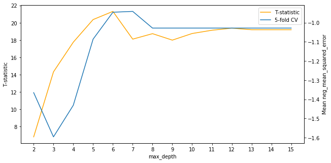
It looks like the best choice for max depth as judged by the T-statistics is slightly lower in the range from 4 to 6 compared to 6 to 8 for cross-validation. It’s worth noting also that the T-statistics for all choices of the hyperparameter are positive, meaning that the mean for the alternative distributions are believed to be higher than the mean of the benchmark distribution.

A test statistic of about 7 corresponds to a p-value of about 0.001, so it’s very clear these models outperform the decision tree with a max depth of 1.

Finally we can sneak a look at performance on the test set to see what value for max_depth actually maximised performance.

neg_mse = []

for max_depth in tree_params['max_depth']:
    tree = DecisionTreeRegressor(max_depth=max_depth)
    tree.fit(X_train, y_train)
    pred = tree.predict(X_test)
    neg_mse.append(-mean_squared_error(y_test, pred))

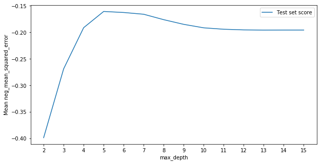
We see the best value for max_depth was just between the estimates given by T-testing and cross-validation at around 5. It seems that cross-validation slightly overfit and T-testing was around the right area.

Model selection extension

Of course we never specified in our hypothesis test that the alternative model is the same model as the benchmark. Let’s investigate if a simple linear regression model with a variable number of polynomial features would outperform the best decision tree we’ve found so far.

As before we will generate our benchmark draws

benchmark_model = DecisionTreeRegressor(max_depth=5)
benchmark_draws = generate_cv_draws(benchmark_model, X_train, y_train, k)

Then generate the candidate draws

model_params = {
    'degree':range(5, 16)
}

models = [make_pipeline(PolynomialFeatures(degree=degree), LinearRegression())
          for degree in model_params['degree']]

t_stats = t_test_grid_cv(models, X_train, y_train, benchmark_draws)

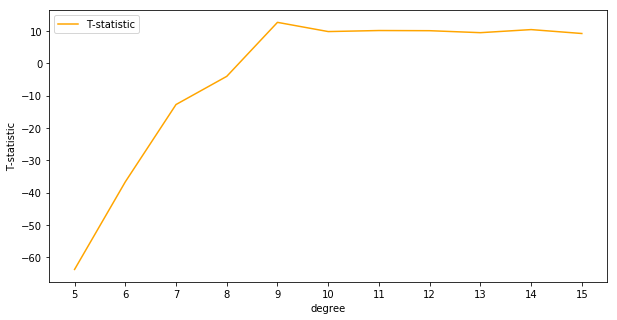
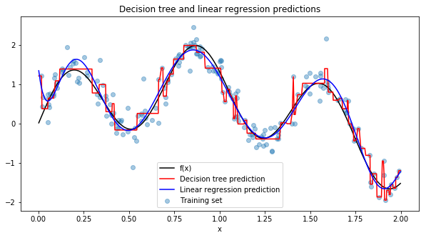
It looks like linear regression with 9th order polynomial terms outperforms the decision tree with very low uncertainty. We can plot the final predictions over the true function \(f(x)\)

References

The content of this article was largely inspired by this post from the Russian data science group ODS. Thanks to Alexander Nikolin for sharing this with me and for translating some spots that seemed to confuse translation software.

@danila_savenkov. 2017. Kaggle Mercedes и кросс-валидация, https://habr.com/company/ods/blog/336168/