Introduction
A few months ago I read this paper from DeepMind that addressed a simple choice of architecture to encourage sensible weights in neural networks when solving problems that at the core are simple arithmetic. Despite the continued hype surrounding neural networks and deep learning in general, some simple problems like this are difficult to generalise past the regions used in a training set.
XOR was a famously difficult problem that stunted developments in perceptrons (the predecessors to what has become neural networks) until Marvin Minsky and Seymour Papert addressed it by applying composition to the model. In a similar vein to the NALU paper, the value added is the proposition of a new architecture since single-layer perceptrons are inherently linear, there’s no way to solve XOR without a multiple layers.
To ensure that we can rely upon neural networks (which are being increasingly used in critical applications) to act sensibly in non-trivial difficult problems, we should ensure it can be flexible enough to solve a wide array of problems, no matter how simple. Additionally, if we know that there is likely a natural arithmetic aspect to a problem, it would undoubtedly help to guide the network through architecting it in a way that exploits that aspect for early approaches.
In summary, the direct goals of this article are to:
- Introduce DeepMind’s NALU architecture
- Outline an implementation (using PyTorch)
- Address some of the drawbacks of the approach
Neural Accumulator (NAC)
Before getting to an architecture that adapts to all four basic arithmetic operations, the paper introduces a unit that tackles addition and subtraction. The design is very simple and uses a clever trick.
In a standard linear layer, the output \(y\) is given by the product of the input \(x\) with some weight matrix \(\mathbf{W}\).
\[ y = \mathbf{W} x \]
In the normal case, we might initialise this matrix \(\mathbf{W}\) with entries that are draws from a normal distribution with a sensible variance (see Xavier and He initialisation). Also during the training process, we might use some form of regularisation to encourage the weights to stay small and prevent us from falling into solutions that fit our data but clearly are not solutions to the underlying problem.
Recall that when we do matrix multiplication, we’re taking a linear combination of the elements in the input vector with coefficients according to each row in \(\mathbf{W}\). If we know that the values in the output vector are just sums or differences of elements in the input vector (i.e. if we know the problem is just addition or subtraction between elements) then the weights should be 0, 1 or -1.
The simplicity in the design of the NAC is to gently push the weights towards
just those values. This is done by using two popular activation functions: tanh
and sigmoid.
Recall that tanh maps \(\mathbb{R} \to [-1, 1]\) and that sigmoid maps
\(\mathbb{R} \to [0, 1]\). Further each function saturates at the endpoints,
meaning that the image of most values in the domain is very close to the edges
of the codomain. We can visualise this by sampling uniformly between -10 and 10
(an arbitrary width) and plotting where the final output lies.
import numpy as np

N_DRAWS = 1000
RESULTS = []

def sigmoid(x):
    return 1 / (1 + np.exp(-x))

for _ in range(N_DRAWS):
    x1, x2 = np.random.uniform(-10, 10, 2)
    RESULTS.append(sigmoid(x1) * np.tanh(x2))

plt.figure(figsize=(8,4))
plt.hist(RESULTS, bins=100)
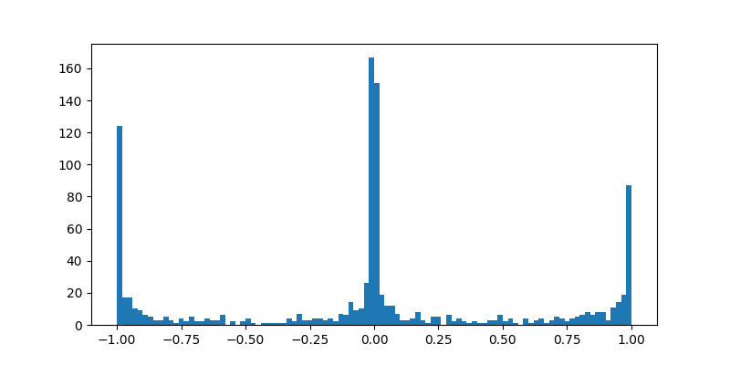
Clearly this pushes the weights towards one of the three values we would expect to see in a weight matrix for an addition or subtraction problem.
Notice that there is a slight bias towards an activation of 0 over the activation of 1 and -1. We can consider the tanh and the sigmoid as a coin flip. To get an activation of 1 or -1 we need the sigmoid output to be 1, therefore half the time the activation is 0 while 1 and -1 occur a quarter of the time each.
Although it might not be directly intended, you could consider this a form of shrinkage and may reduce bias in the model.
To use this observation, we simply apply the same transformations when constructing the weight matrix \(\mathbf{W}\). DeepMind choose to structure it in this manner.
\[ \mathbf{W} = \text{tanh}({\mathbf{\hat{W}}}) \odot \text{sigmoid}({\mathbf{\hat{M}}}) \]
where \(\odot\) is the Hadamard or element-wise product operator. Here \(\mathbf{W}\) is the output weight matrix whose elements will be biased towards -1, 0 and 1 and \(\mathbf{\hat{W}}, \mathbf{\hat{M}}\) are underlying latent matrices. All three matrices have the same shape, \(M \times N\), where \(N\) is the input dimension and \(M\) is the output dimension.
We can apply backpropogation during training as per usual since our transformation is differentiable. This also concretely bounds the range of values in \(\mathbf{W}\) so we might posit it could stabilise the training process also. Otherwise, this is effectively a drop-in replacement for a traditional linear layer.
Neural Arithmetic Logic Unit (NALU)
A useful and simple identity of logs is the following.
\[ \log (a \times b) = \log a + \log b \]
Although it was much before my time, this used to be heavily exploited for any kind of multiplication and division prior to computers reaching the masses by using slide rules. NALU’s exploit this exact same identity. We’ve established a method for addition and subtraction, so now we repeat this process just in the log-space.
We’ll call the output of the regular NAC \(a\) and the output of the NAC that operates in log-space \(m\). From before, \(a\) is the simple product
\[ a = \mathbf{W} x \]
where \(\mathbf{W}\) is the same weight matrix as discussed before. For \(m\), we take the log of our input vector, multiply by the weight matrix and take the exponent to return to level-space.
\[ \tilde{m} = \exp ( \mathbf{W} \log (x) ) \]
One issue we quickly find is that since we have no bounds on the elements of \(x\), we can’t guarantee they are positive values. Therefore instead of \(\tilde{m}\) we use,
\[ m = \exp ( \mathbf{W} \log (|x| + \epsilon) ) \]
where \(|x|\) is the vector containing the absolute value of each element of \(x\) and \(\epsilon\) is some small value (e.g. 1e-8). We use the common broadcasting notation here but mean that \(\epsilon\) is added element-wise to \(|x|\).
Now we have an output that utilises addition/subtraction \(a\) and one that uses multiplication/division \(m\). DeepMind suggest a third output \(g\) that acts as a gate to control which of these outputs is used by the layer.
We use a similar trick to guarantee that the elements of the gate \(g\) are in \([0, 1]\).
\[ g = \sigma (\mathbf{G} x) \]
Therefore our final output interpolates between \(a\) and \(m\) using \(g\).
\[ y = g \odot a + (1 - g) \odot m \]
Note that \(g\) is applied element-wise. This means that the final vector output from the layer might include some elements that are produced from addition/subtraction and some that are produced from multiplication/division.
How do we implement the layers?
Now that we’ve established the structure of the network, the implementation is relatively straightforward. We’ll use PyTorch in this example but TensorFlow or any other similar library will work just fine. We’ll start with a NAC. First let’s look at the code and walk through it afterwards.
import torch
import torch.nn as nn

class NeuralAccumulator(nn.Module):
    def __init__(self, input_dim, output_dim):
        super().__init__()

        self.what = nn.Parameter(torch.empty((input_dim, output_dim)))
        nn.init.xavier_normal_(self.what)

        self.mhat = nn.Parameter(torch.empty((input_dim, output_dim)))
        nn.init.xavier_normal_(self.mhat)

    def forward(self, x):
        w = self.what.sigmoid() * self.mhat.tanh()
        return x @ w
This is pretty simple. We initialise the matrices \(\mathbf{\hat{W}}\) and
\(\mathbf{\hat{M}}\) randomly (in this case just by using Xavier initialisation)
and when evaluating an input we compute the matrix \(\mathbf{W}\) using the
formula discussed previously and compute the matrix product with the input
vector \(x\). Note that the @ operator in python is syntactic sugar for matrix
multiplication in common libraries (PyTorch, Numpy, TensorFlow, etc).
That’s really all there is. PyTorch makes it quite easy to compose layers together, so we construct the NALU by building on from the NAC.
In this instance we deviate slightly from the design of the NALU in the original paper. Here we’ll create two separate NAC’s: one for the level space and one for the log space. In contrast, the original paper depicts the weights for each space as being shared.
class NeuralArithmeticLogicUnit(torch.nn.Module):
    def __init__(self, input_dim, output_dim):
        super().__init__()

        self.level_nac = NeuralAccumulator(input_dim, output_dim)
        self.log_nac = NeuralAccumulator(input_dim, output_dim)

        self.G = nn.Parameter(torch.empty((input_dim, output_dim)))
        nn.init.xavier_normal_(self.G)

    def forward(self, x):
        a = self.level_nac(x)
        m = (self.log_nac((torch.abs(x) + 1e-7).log())).exp()
        g = x @ self.G
        return g * a + (1 - g) * m
Again this is already very close to just writing the formulas from the previous sections. In this case we’ve chosen to set \(\epsilon=10^{-7}\). This is arbitrary and shouldn’t matter too much (any sufficiently small number will do just fine).
One section that should be examined closer is the calculation of the weighted product between \(a\) and \(m\).
return g * a + (1 - g) * m
Suppose the output dimension is 5. Then the shape of \(g\) is torch.Size([5])
while the shape of \(a\) and \(m\) are torch.Size([?, 5]). Commonly we use ? to
denote the mini-batch dimension. Therefore we cannot take the elementwise
product since \(g\) doesn’t match the shape of either \(a\) nor \(m\). What is
happening here is we are broadcasting the product across the first dimension.
That is we take the element-wise product along each step in first dimension.
Mystery arithmetic problem
To do complete a further investigation, we need a test problem to apply the network to. We’ll use something similar to one of the examples in the paper which we’ll call the “mystery arithmetic problem”.
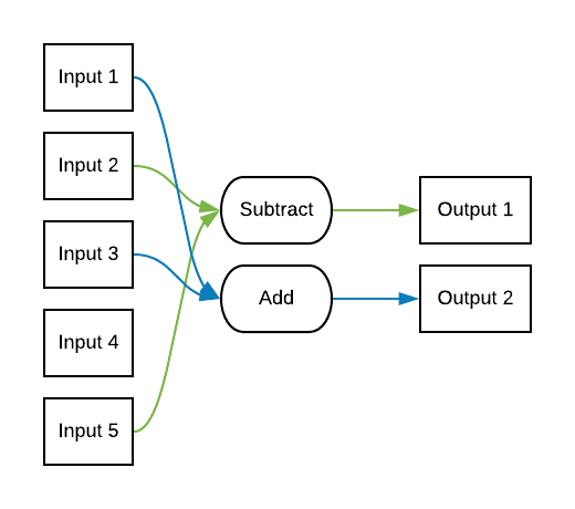
In this problem suppose we have \(n\) inputs and \(m\) outputs. Each output is randomly associated with two of the inputs and one of the four binary arithmetic operators. For example one instance of the problem might be described as the following.
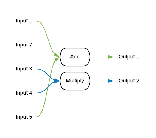
While in another randomly generated problem, the solution might look like this.
Given a configuration, we can generate training and test data easily. Here we show an example implementation to generate configurations and the solution to an input vector given a configuration.
from enum import Enum, auto
from random import choice, sample

class Operation(Enum):
    ADD = auto()
    SUBTRACT = auto()
    MULTIPLY = auto()
    DIVIDE = auto()

def generate_configuration(in_dim, out_dim):
    """
    Returns a list of length `out_dim` containing tuples in the form of (i, j, o)
    where i and j are indices and o is an operation.
    """

    indices = range(in_dim)
    operations = [Operation.ADD,
                  Operation.SUBTRACT,
                  Operation.MULTIPLY,
                  Operation.DIVIDE]

    configuration = []

    for _ in range(out_dim):
        i, j = sample(indices, 2)
        o = choice(operations)
        configuration.append((i, j, o))

    return configuration
As a small note, we will omit division problems from the training and test sets used in the rest of the article to stablise some of the training (since we use the same interval that includes numbers very close to zero). In the paper they test each of these operations separately but here we generate a combination of them in a single instance of the problem.
def compute_minibatch_solution(minibatch, configuration):
    """
    Given a configuration and minibatch (as a (batch_size, in_dim) shaped numpy
    array) inefficiently computes the solution to the mystery arithmetic problem.
    """

    minibatch_solution = []

    for x in minibatch:
        x_soln = []

        for i, j, o in configuration:
            if o == Operation.ADD:
                x_soln.append(x[i] + x[j])
            elif o == Operation.SUBTRACT:
                x_soln.append(x[i] - x[j])
            elif o == Operation.MULTIPLY:
                x_soln.append(x[i] * x[j])
            elif o == Operation.DIVIDE:
                x_soln.append(x[i] / x[j])
            else:
                raise TypeError(f'Unknown operation {o}')

        minibatch_solution.append(x_soln)

    return np.array(minibatch_solution)
We can use these to generate a training set by generating a random array populated with uniformly distributed random numbers from \([-10, 10]\) and then computing the solution for a configuration. The implementation to solve the problem using the true configuration is not intended to be at all efficient or fast. There is likely a better way to represent the configuration that would allow for vectorisation.
in_dimension = 100
out_dimension = 10

training_set_size = 1000
test_set_size = 1000

conf = generate_configuration(in_dimension, out_dimension)

X_train = np.random.uniform(-10, 10, (training_set_size, in_dimension))
y_train = compute_minibatch_solution(X_train, conf)
We will use a wider range for the values of the test set, the interval \([-50, 50]\) in order to expose any networks that have overfit the smaller interval.
X_test = np.random.uniform(-10, 10, (test_set_size, in_dimension))
y_test = compute_minibatch_solution(X_test, conf)
Performance evaluation
Let’s compare the performance against a vanilla dense network with ReLU activation.
import torch.nn.functional as F

class VanillaNetwork(nn.Module):
    def __init__(self, input_dim, output_dim):
        super().__init__()
        self.fc = nn.Linear(input_dim, output_dim)

    def forward(self, x):
        return F.relu(self.fc(x))
We’ll now train using the following methodology:
- 250 epochs with a batch size of 32
- Adam with a learning rate of 0.001
- MSE loss
import pandas as pd
from torch.optim import Adam
from torch.utils.data import TensorDataset, DataLoader

n_epochs = 250
lr = 0.001
batch_size = 32

train_dataset = TensorDataset(torch.from_numpy(X_train).float(), torch.from_numpy(y_train).float())
train_loader = DataLoader(dataset=train_dataset, batch_size=batch_size)

test_dataset = TensorDataset(torch.from_numpy(X_test).float(), torch.from_numpy(y_test).float())
test_loader = DataLoader(dataset=test_dataset, batch_size=batch_size)

networks = {'vanilla': VanillaNetwork(in_dimension, out_dimension),
            'nac': NeuralAccumulator(in_dimension, out_dimension),
            'nalu': NeuralArithmeticLogicUnit(in_dimension, out_dimension)}

training_loss = pd.DataFrame()
test_loss = pd.DataFrame()

for net_name, net in networks.items():
    print(f'Beginning training for {net_name}')
    optimizer = Adam(net.parameters(), lr=lr)
    train_loss_history = []
    test_loss_history = []

    for n_epoch in range(1, n_epochs+1):
        train_losses = []
        test_losses = []

        for x_batch, y_batch in train_loader:
            loss = F.mse_loss(net(x_batch), y_batch)
            optimizer.zero_grad()
            loss.backward()
            optimizer.step()
            train_losses.append(loss.detach().item())

        with torch.no_grad():
            for x_batch, y_batch in test_loader:
                loss = F.mse_loss(net(x_batch), y_batch)
                test_losses.append(loss.detach().item())

        if n_epoch % 50 == 0:
            print(f'Epoch {n_epoch}, MSE = {loss.detach():.4f}')

        train_loss_history.append(np.mean(train_losses))
        test_loss_history.append(np.mean(test_losses))

    training_loss = pd.concat([training_loss, pd.DataFrame({net_name: train_loss_history})], axis=1)
    test_loss = pd.concat([test_loss, pd.DataFrame({net_name: test_loss_history})], axis=1)

training_loss['epoch'] = np.arange(n_epochs) + 1
test_loss['epoch'] = np.arange(n_epochs) + 1
And we can look at loss curve for the training set.
import seaborn as sns

melted_loss = training_loss.melt(id_vars='epoch',
                                 value_name='MSE Loss',
                                 var_name='Architecture')

sns.relplot(x='epoch', y='MSE Loss',
            hue='Architecture', kind='line',
            height=5, aspect=8/5,
            data=melted_loss);
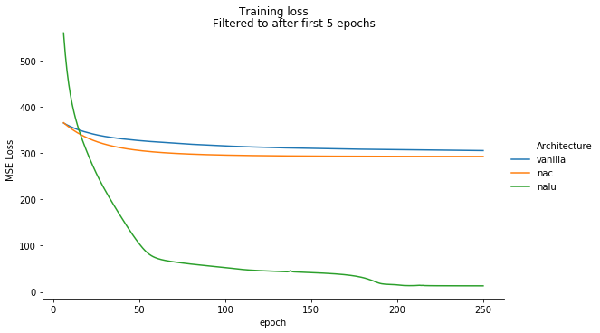
We can see that the NALU dominates both the Vanilla and NAC networks, as expected. The NAC befores better than the Vanilla architecture (since it is able to solve both the addition and subtraction cases perfectly) but cannot fit the multiplication and division cases.
Let’s also check the test loss curve to ensure we have not overfit or had any strange abberations in our training loss.
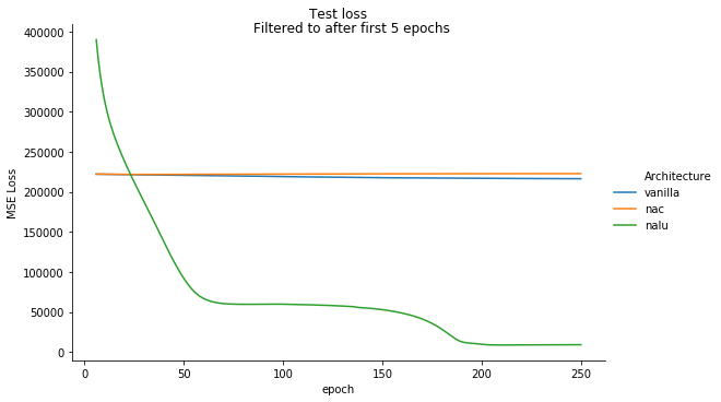
We see no significant change for the performance of the NALU. It indeed looks to have come close to the exact solution (but it not quite as we will see in the next section). In contrast, the NAC and Vanilla networks have swapped places, with the NAC appearing to have overfit slightly. If we looked closer we might expect to see most of this loss coming from the parts of the vector that are products rather than addition or subtraction.
Caveats
When we compute the sum/difference in the log space, we are forced to throw away the sign of the elements in the vector in order to take the log. This restricts us and we actually cannot learn to solve some problems as a result. For example, suppose the system we are trying to fit takes the product of the first and second elements in a vector. For example,
\[ x = \begin{bmatrix} 1.5 \\ 2 \\ 2.5 \end{bmatrix} \to 3 \]
We can model this by taking the sum in the log space. This would be equivalent to the following.
\[ \exp \left ( \begin{bmatrix} 1 & 1 & 0 \end{bmatrix} \cdot \ln(x) \right ) \]
and indeed this would give the correct result in this case. However, suppose our input was instead the following.
\[ x = \begin{bmatrix} 1.5 \\ -2 \\ 2.5 \end{bmatrix} \to -3 \]
Since we actually take the absolute value of \(x\), we throw away the signs here and cannot compute the correct product.
We could address this by creating another mechanism in the layer to adjust the output based on the signs of the input, but this is not done in the paper.
References
Trask, A., Hill, F., Reed, S. E., Rae, J., Dyer, C., & Blunsom, P. (2018). Neural arithmetic logic units. In Advances in Neural Information Processing Systems (pp. 8035-8044).
Xavier and He Normal (He-et-al) Initialization, mc.ai retrieved on January 5th 2020.
Changelog
| Date | Changes |
|---|---|
| January 14th 2020 | Published original version |
| January 28th 2020 | Cleaned up training and test loss graphs |