Introduction
In this article we’ll review Q-learning and walk through a subtle improvement that leads to Double Q-learning and better policies. We’ll then look at this in action, and compare the two methods on a toy problem.
Reinforcement learning refresher
In this article I assume a familiarity with reinforcement learning and the standard Q-learning algorithm. In this section I’ll provide a brief review of the basic terminology, which you can feel free to skip if you’re comfortable in doing so.
Reinforcement learning is a field of machine learning that has risen in popularity particularly over the last 10 years riding on the achivements in areas like computer Go and computational chemistry. There are a few core elements in the field.
The environment is a model or representation of the current state of the world. In this article you can assume it is discrete and fully observable (although in partial information games like poker, this is not the case). The agent follows a policy which maps each state to an action the agent makes when interacting with the environment. This action then produces a new observation representing the new state of the environment and a scalar reward.
The goal of reinforcement learning is to find a policy for the agent that maximises the cumulative rewards emitted from the environment. Q-learning is one particular approach that estimates a policy without requiring perfect knowledge of the dynamics of the environment (e.g. the probability transition matrix of an MDP).
Q-learning algorithm refresher
Q-learning generates a policy using a table of bootstrapped “q-values” that correspond to the quality of an action. Concretely, they are a mapping from a state \(s\) and action \(a\) to a scalar. If \(S\) is the set of states and \(A\) the set of actions then,
\[ Q : S \times A \to \mathbb{R} \]
The optimal q-value function, denoted \(Q^*\), satisfies something called the Bellman equation and implies that \(Q^*(s,a)\) is equal to the expected future rewards if the agent plays \(a\) in \(s\). If we know \(Q^*\) then the trivial policy derived from it is to choose \(a\) that maximises \(Q(s,a)\) given our current state \(s\). We commonly denote a policy with \(\pi\).
\[ \pi^* : S \to A \] \[ \pi^*(s) = \underset{a}{\text{arg max }} Q^*(s, a) \]
If we assume there are a finite number of states and a finite number of actions then \(S\) and \(A\) are finite sets. This means we can think of \(Q\) as a lookup table. The issue now is that we don’t know \(Q^*\) and have to estimate it over time as we observe rewards and transitions between states as the agent makes actions. At time \(t\) the estimated q-value function is denoted \(Q_t\) and the corresponding policy \(\pi_t\).
Q-learning iteratively improves \(Q_t\) using the following update equation applied with a new transition from \(s\) to \(s^{\prime}\) after the agent took an action \(a\) leading to a reward of \(r\).
\[ Q_{t+1}(s, a) := Q_t(s, a) + \alpha \left ( r + \gamma \thinspace \underset{a^{\prime}}{\text{max }} Q_t(s^{\prime}, a^{\prime}) - Q_t(s, a) \right ) \]
Where \(\alpha \in (0, 1]\) is a scalar learning rate and \(\gamma \in [0,1]\) is a scalar discount factor (you don’t need to worry too much about either of these). This looks a little scary but really it’s just linear interpolation between our old estimate \(Q_t(s, a)\) and our new estimate \(r + \gamma \thinspace \underset{a^{\prime}}{\text{max }} Q_t(s^{\prime}, a^{\prime})\). We can rewrite the update equation like so,
\[ Q_{t+1}(s, a) := (1 - \alpha) \thinspace Q_t(s, a) + \alpha \left ( r + \gamma \thinspace \underset{a^{\prime}}{\text{max }} Q_t(s^{\prime}, a^{\prime}) \right) \]
to illustrate this point. The greater \(\alpha\) is, the more weight we put on our
new estimate of the q-value. It is shown by
A closer look at our estimator
Until now we’ve looked at the problem from a specific and applied point of view. Let’s now take a step back and look at a particular part of the update equation and see if we can improve upon it.
We’ve already stated that our current estimate with the new transition is given by
\[ r + \gamma \thinspace \underset{a^{\prime}}{\text{max }} Q_t(s^{\prime}, a^{\prime}) \]
This expression tells us that we’re moving \(Q_{t+1}(s, a)\) towards the reward we just received \(r\) plus the expected cumulative rewards in the future. It’s important to distinguish between the estimator and the parameter of the latter part. The value we’re trying to estimate is
\[ \underset{a^{\prime}}{\text{max }} Q^*(s^{\prime}, a^{\prime}) \]
and the estimator we’re using is
\[ \underset{a^{\prime}}{\text{max }} Q_t(s^{\prime}, a^{\prime}) \]
A more general formulation of this problem is given a set of \(k\) random variables \(X = \{X_1, \ldots, X_n\}\) find the maximum expected value of the random variables. The issue here is that the choice of the estimator used in Q-learning is tied to the value of the estimator. Estimators with unusually large values at time \(t\) are chosen more frequently, and this leads to an exaggeration of the true value of the next state. Therefore we end up being optimistic, which we’ll later see can lead to worse policies before convergence to \(Q^*\). This issue is called maximisation bias.
A key contribution by
| Action | \(Q_t^1(s, a)\) | \(Q_t^2(s, a)\) |
|---|---|---|
| \(a_1\) | -4.9 | -2.3 |
| \(a_2\) | 2.3 | 4.3 |
| \(a_3\) | 4.0 | 3.5 |
With regular Q-learning we choose the action with the highest q-value and use that q-value as the estimate of the value. Here if we use \(Q_t^1(s, a)\) that gives us \(a_3\) for an estimated value of 4.0. With Double Q-learning we still select \(a_3\) but we use the value from \(Q_t^2(s, a)\) giving us an estimate of 3.5.
It can be shown that this is also a biased estimator, but with a negative bias rather than a positive bias as with regular Q-learning.
Illustration of maximisation bias
We will use the example given in
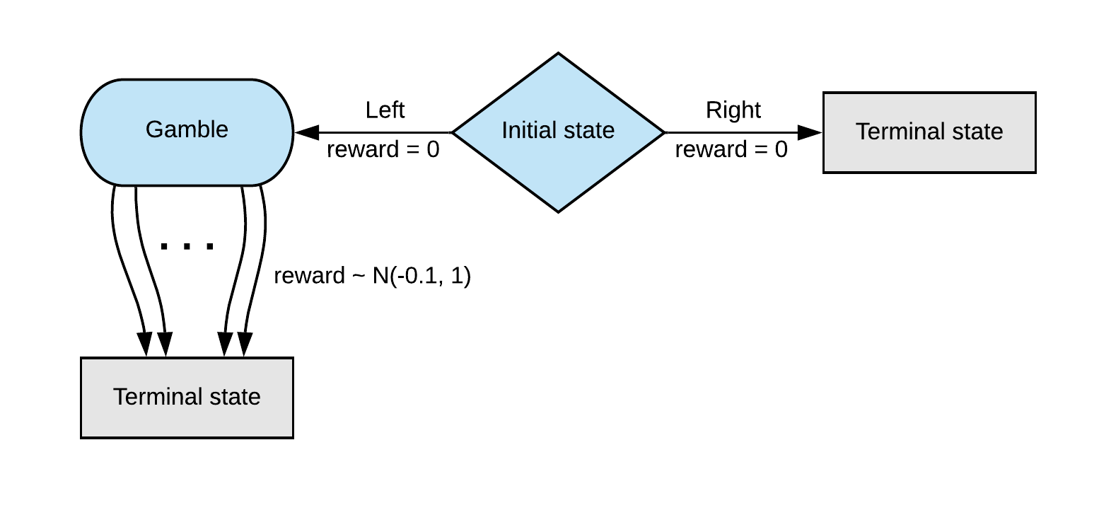
When we start the game we have two options avaliable to us. If we play Right
the game immediately ends and we receive a reward of 0. If we play Left we
move to another state Gamble and receive a reward of 0. From Gamble we can
choose one of \(k\) different actions. Upon selecting one of these actions the
game ends and we receive a random reward drawn from a \(\mathcal{N}(-0.1, 1)\)
distribution.
It’s important to remember that we learn our policy without knowing the
structure of this MDP (otherwise we already know to always choose Right).
Let’s compare the policies learnt with Q-learning and Double Q-learning when
playing in this environment. Below we post the percentage of time the algorithm
chooses to take Left from the initial state. The optimal policy plays Left
5% of the time due to detail in our training process 1. The curve
is created by repeating the training process from scratch many times to smooth
it out. Below is the graph for \(k=4\).
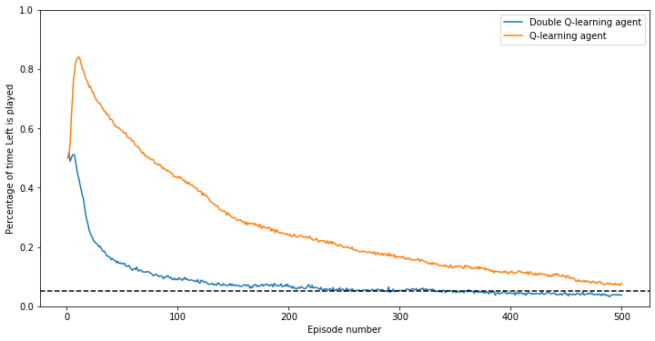
Given our initial estimates of the q-values we are indifferent to either Left
or Right so we take Left about half the time. Soon after, Q-learning begins
to take Left much more frequently. This is usually caused by being lucky on
one of the \(k\) actions from the Gamble state, causing our q-value to be
positive and therefore greater than the value of taking Right. Over time as we
collect more samples our estimate gradually begins to reflect the actual reward
distribution which has a mean of -0.1.
In contrast, we see that Double Q-learning very quickly adjusts and is not
affected by any lucky draws from actions taken in the Gamble state. Double
Q-learning performs much better in this game, and empirically this has been the
recurring theme across many games. Even though both methods converge to \(Q^*\)
the policies in the meantime tend to be better in most games when being
pessimistic. This is particularly remarkable since when Double Q-learning splits
the samples into two groups, the variance of the estimators grows. This means it
has lower sample efficiency, but despite this, removing the optimism from
Q-learning still usually outweighs this disadvantage.
Review
We have reviewed the basic Q-learning algorithm as an approach to reinforcement learning. We saw that you can view the update equation as simple linear interpolation between the existing estimate and a new observation of the q-value. We looked at how you can improve the forward looking estimate of future cumulative reward, and how the estimator chosen for this quantity is tied to its value. This is addressed by Double Q-learning which we saw in the dummy problem tends to exhibit much better policies whilst maintaing the same convergence property towards the optimal q-value function \(Q^*\).
<~/org/braindump/roam/bibliography/papers.bib>
-
We use epsilon-greedy exploration while training for both algorithms with epsilon fixed at 90%. Therefore optimally
Rightis always choosen in the greedy step, and sinceLeftis chosen 50% of the time in the explore step, an optimal policy playsLeft5% of the time. ↩︎