Introduction

Recently I’ve been motivated to investigate generative models, of which the most popular is currently GANs. The best way I could think of learning about GANs in deeper detail (since I’m interested in tweaking them later in some applied cases) is to implement them myself, and solve the bugs and issues that arise in practice myself.

In this article I’ll use PyTorch and a framework that helps simplify training called PyTorch Lightning (Falcon, 2019). PyTorch Lightning allow separation of training code from network architecture code. It also exposes useful callback methods to quickly add different logging or debugging which can be useful when training GANs, which is often a non-trivial process.

Hence I want to provide a short reiteration of my path through implementing common GAN architectures and some of the issues I faced. You can look at the history of the code in this repo. I’d encourage you to try follow along if so inclined, the examples could even be run on a CPU with some patience. In the case you don’t have patience you could also use Google Collab which gives you a free GPU (or TPU) to use.

Starting with a MLP GAN

Let’s start with the most basic realisation of a GAN: two fully connected neural networks each trying to trip the other up. Just fully linear layers with ReLU and binary cross entropy loss. Some might just call this a vanilla GAN. For the target distribution we will use something that we know should work based on literature and endless stream of blog posts, MNIST.

I have a basic implementation here you can run (I encourage you to follow along yourself and make the corresponding changes to the code discussed throughout the post). Let’s generate one of those oh so famous plots showing a few vectors of noise put through the generator over time. We’ll go for 100 epochs here.

Hm, that doesn’t look good. Although there are vague circular outlines towards the end of the video, it’s almost entirely noise. As a reminder, the target distribution, MNIST, looks like this.

So okay, all our matrices are the right shapes but clearly there’s some poor conditioning here and we’re not converging to any sort of meaningful result.

The first thing we could try is actually read the original research and compare our network with what’s described in (Goodfellow et al., 2014). The blocks I’m using at the moment include

A linear layer
ReLU activation
Batch norm

and we run through three blocks before resizing to the dimensionality of the image or squishing down to a probability (using tanh or sigmoid as the final output respectively). (Goodfellow et al., 2014) mentions using Dropout for normalisation as their paper actually came out a year before (Ioffe & Szegedy, 2015) where batch norm was introduced. So we could try changing our blocks to look like

A linear layer
ReLU activation
Dropout

This change was made in ba00ce3. Let’s run another 100 epochs with this style of block for both the generator and the discriminator.

Wow this is looking great now! The samples drawn definitely resemble digits. We can see it’s learnt that the background is mostly black and the foreground should have a white digit-like figure. It definitely looks like dropout is the better choice here. However, we can still see some noisy white spots fringing around the digits. The internal dimension for the generator here is set to 512, which is just an eighth of the dimension of the output image (our MNIST images are preprocessed 64x64) so it might be expected that there’s still some noisy in the mapping.

So now we’ve got one model that seems to converge well, and one that totally failed. PyTorch Lightning gives us Tensorboard logging for free, so let’s take advantage of that and use this as a learning experience and compare the loss and gradients for these networks.

First the loss. The blue line here the network using batch norm and the pink line is the network using dropout.

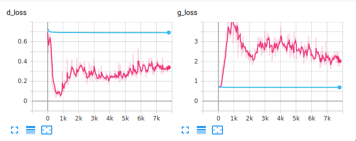
We can see that for the batch norm network the losses converged straight to \(\ln 2\) which is the stable loss value for GANs when viewing the training process as convergence to a Nash equilibrium. On the other hand, we see that the dropout network actually saw the discriminator take the lead and the generator had to play catch up. We could posit that perhaps the generator in the dropout network was able to qualitatively improve due to discriminator being more accurate, which means in turn the generator has a better signal for how to improve its fakes. Once the batch norm network hit its equilibrium loss for the two networks, it might have struggled to move the weights significantly from that minima.

Now, let’s have a look at the gradient logging added in 14a0428. Here we’ll look at the gradients of the last weight layer in the discriminator. Browsing through the histograms for each of the layers one that stood out to me was the weights in the last layer of the discriminator. These are the weights in the linear layer that projects the discriminator network activations to scalars, which are in turn mapped to \([0,1]\) with a sigmoid activation.

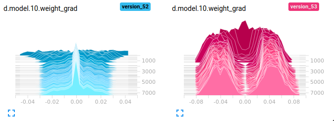
Here we can see that the gradients in the batch norm network shrunk towards zero, over time. This makes the updates to the weights very small, and causes the network to freeze up. This partially explains why you may have thought the video of the samples drawn from the batch norm network wasn’t moving (I was worried my ffmpeg line hadn’t worked at first). The bimodal distribution and magnitude of the gradients (look at the x-axis!) in the dropout network clearly signal that the network is not succumbing to vanishing gradients.

I’m happy with this result for a simple fully connected GAN, on a simple dataset.

Pokemon!

Let’s next try our simple fully connected architecture on a dataset with more than one channel - pokemon sprites. This dataset was also explored in (Weng, 2017) which also provides a fantastic review of the history of GANs including better commentary on theoretical changes.

I added a small data loader to scrape images off a website in eca3062. To train on the pokemon dataset is as simple as running.

python src/main.py --gpus -1 --dataset pokemon

Ehhh that’s not too great of a result. We can see it’s roughly learnt there should be a dark background and a figure in the middle, but not much more than that. We can also see a lot of noisy pixels over the entire image. Let’s move onto a more complicated architecture and continue with this dataset for testing as the limitation here is likely the capacity of the model, rather than anything training related (I tested this by increasing the latent dimension and image size, with results almost identical to what’s shown here).

Using convolutions with DCGAN

The next architecture we’ll look at is DCGAN (DC here stands for deep convolutional). (Radford et al., 2015) extend the basic idea of a GAN by adapting the network architecture to follow the immensely popular CNNs that had just begun to take over ImageNet at the time. There’s no change to the fundamental training regime (we still have a generator and a discriminator) we just use (de)convolutional layers in place of fully connected layers.

Before going back to basics with the original GAN above, I had a stab at implementing a DCGAN. I’ve copied the code over in 82e372d and we’ll work through cleaning it up and making sure everything works.

python src/main.py --gpus -1 --network dcgan --dataset pokemon --max-epochs 50

Great this looks like an improvement on the fully connected GAN. Note that the noise around the figures is greatly reduced now. We have still learnt that there should be a figure in the middle, but the network doesn’t seem to be able to decide on the hue of it.

In d646c6f I do some refactoring to standardise the structure of blocks in the generator and discriminator and also make the number of filters and blocks configurable. What we can do now is compare the samples from networks with varying capacity, to see if that’s the limitation at hand. Let’s try moving from 16 filters and 3 blocks to 32 filters and 5 blocks as well as increasing the size of the images to 128x128.

python src/main.py ... --img-size 128 --n-filters 32 --n-blocks 5

RuntimeError: size mismatch, m1: [32 x 2048], m2: [8192 x 1] at /pytorch/aten/src/THC/generic/THCTensorMathBlas.cu:283
Exception ignored in: <function tqdm.__del__ at 0x7fd2be9102f0>

Whoops, a quick scan back through the code and it looks like the linear layer of the discriminator wasn’t adjusted to change size with the number of blocks we use. A quick fix in eb73ef1 and making the filters and blocks configurable in 83907cd yields the following

This seems to be only a marginal improvement from the last DCGAN. We see very fine detail now (in fact some of the lines are very thin) and the blobs are centralised with little fringing. There is some heterogeneity in the blob size, but the hue of each of the figures is approximately the same.

Transposed convolutions

If you look at my code you’ll see up to this point I have used nn.Upsample in the generator followed by a convolutional layer with a kernel size of 3, stride of 1 and padding of 1. The key point to note here is the unsampling actually uses nearest neighbouring interpolation by default. Another option is to use transposed convolutions or fractionally strided convolutions. This takes advantage of the fact that a kernel produces two matrices: one from a big image to a small image (roughly speaking) and another that does the reverse. Since we’re upsampling, if we transpose the matrix generated from the kernel, we can learn the weights used in the interpolation, rather than just falling back on nearest neighbours. I suggest (Dumoulin & Visin, 2016) for a more detailed walk through of the arithmetic used here. I swap to this alternative method of upsampling in 429209e. Let’s have a look at a run using the same settings as the above to see if there’s much of a difference.

You can see that the picture is totally grainy, compared to the last DCGAN sample video and this makes sense when you think about the change how interpolation works. With the last video the initially small image projected from the random vector is repeatedly upsampled using nearest neighbour interpolation. That means that pixels are blended together, causing the psychedelic-esque patterns at the start of the video. Conversely, for transposed convolutions the weights are random initially, causing the graininess seen above.

Overall we see it failed to converge over 50 epochs. As I was watching the network train I noted that the discriminator got way ahead of the generator here. Let’s look at the loss curves.

Not great. We’ve added a lot of capacity to the generator by freeing up the interpolation which is good in theory as in means we should be able to produce a wider variety of images, but not if the discriminator dominates the generator first (as we lose meaningful gradients). Let’s try updating the generator 5 times for each time we update the discriminator to see if that helps. Added in 5c182ec.

Well at least that failed slower? The samples are omitted as they are similar to before.

We might have to try another approach.

Swapping out the loss with WGANs

(Arjovsky et al., 2017) propose the usage of the Wasserstein distance function as an alternative to binary cross entropy loss. They illustrate that in many cases the KL divergence and JS divergence (not covered here) between high dimensional distributions is undefined, making it extremely difficult to optimise for. This is the reason a popular approach is to add Gaussian noise to real samples to expand the support of the distribution, making KL and JS tamable. Wasserstein distance is a simpler approach, and often leads to less complicated and more stable training.

In 4132ad1 I add an implementation using the same generator and discriminator (now called a critic) as in the DCGAN. Let’s look at an example runs on the Pokemon and MNIST datasets.

The first thing to note is that some of the training is starting to chug along here. The Pokemon clip is actually played back 2.5x faster than the other samples up to this point (even when training at a learning rate of 1e-4). However, we see a lot of diversity in the samples from both clips, with reasonable quality.

If we look at the loss curves for the Pokemon run, we can see some strange results.

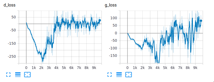
In the implementation so far, I’ve chosen to follow what many open source implementations do in replacing the sigmoid activation of the critic with an unbounded linear activation. This leads to the huge loss we see above. Note as well the default here is to train using gradient penalty (Gulrajani et al., 2017), with \(\lambda=10\). This means that the loss from our average scores from the critic far outweighs the gradient penalty, potentially causing the instability after the first third of training. At this level, the optimiser might as well ignore the gradient penalty term altogether, since it’s such an insignificant part of the overall loss.

Where from here?

There’s lots of directions you could take from here. Here’s a short list.

Use a bigger dataset

It’s quite possible that due to the pokemon dataset being relatively small (just a few hundred images) the GANs above are simply don’t have the sample efficiency to reasonably fit the distribution of the images. A common choice in literature is the LSUN bedrooms dataset but there’s many other classes you could use as well.

Use a better generator and critic

There’s been a lot of success with using deeper and larger resnet architectures. Why not try and replace the standard convolutional layers with skip connections?

Try out different non-linearities and hyperparameter choices

PyTorch lightning makes it easy to plug and play with a variety of logging libraries that make it easier to compare which hyperparameter choices are effective. Try using test-tube, wandb or just regular TensorBoard.