Auto-regressive time series in R

Introduction

In this post we’ll go over auto-regressive time series. What they are, what they look like and some properties they exhibit. Throughout the post we’ll use small snippets of R to plot processes and visualisations.

What are autoregressive time series?

An auto-regressive time series is a stochastic process in which future values are modelled by a linear combination of some number of previous values of the same process. In other words, a series which is regressed on itself in order to find coefficients that relate its past values to its future values. The order of an auto-regressive series is the number of lags used in the model. If the previous four values of the process are used then we say the process is a fourth order auto-regressive process, or $AR(4)$ for short.

In general, an auto-regressive process using the previous $n$ lags is denoted as an $AR(n)$ process. The general form of $S_t$, the value of an $AR(n)$ process at time $t$, is

\[ S_t = \beta_0 + \sum_{k=1}^n \beta_k S_{t-k} + \varepsilon_t \]

where $\varepsilon_t \sim \text{i.i.d. } \mathcal{N}(\mu, \sigma^2)$ is a random disturbance or error. The coefficients $\beta_0, , \ldots, , \beta_n$ express the relationship between future values and lags. Since this is the typical setup for linear regression, under relatively weak assumptions we can make an unbiased estimate of the future values of the process. The most important of these assumptions is that the lags are strictly exogenous, meaning that the expectation of the error at each time is equal to zero conditional on all lags. Concretely,

\[ \mathbb{E}[\varepsilon_t | S_j] = 0, , \forall j \in 1, , \ldots, , t \]

This is a stricter assumption than contemporaneous exogeneity in which errors have a conditional expectation of zero given just the previous $n$ lags.

What do they look like?

As we will see, auto-regressive processes can fit a variety of cyclic and seasonal patterns. We’ll implement a function to generate draws from an $AR(n)$ model with a particular set of coefficients in R.

ar_n <- function(betas, n_steps) {
  y <- c(0)
  for (i in 2:n_steps) {
    next_y <- rnorm(1)
    for (j in 1:min(length(betas), length(y))) {
      next_y <- next_y + (betas[j] * y[length(y)-j+1])
    }
    y <- c(y, next_y)
  }
  y
}

A common example of a process is a random walk, in which the current value of the process is equal to the previous value plus a random jitter (usually drawn from a normal distribution). This can be modelled as an $AR(1)$ process with $\beta_0 = 0$ and $\beta_1 = 1$. This gives us the following expression for the value at time $t$

\[ S_t = S_{t-1} + \varepsilon_t \]

We can also plot a draw from this process using the built-in plot.

x <- seq(1, 200)
plot(x, ar_n(c(1), 200), type='l')

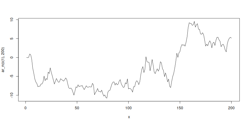
While it may appear that there is trending in the series, there is only completely random movement. At any point the process is just as likely to move up or down, regardless of its previous trend. That is, it is memoryless. We can plot another $AR(1)$ process with a smaller coefficient, say $\beta_1 = 0.5$.

plot(x, ar_n(c(0.5), 200), type='l')

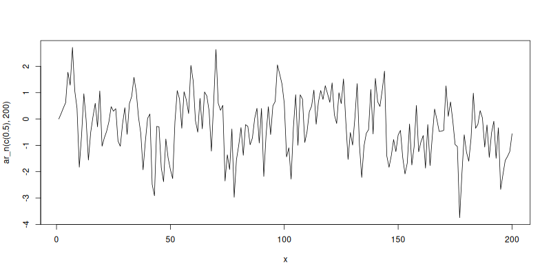
Here in constrast to the random walk the process tends to oscillate around its starting value of 0 and never trend too far in a single direction. We’ll look more at this property in detail in the next section.

How about high order auto-regressive processes? Let’s try an $AR(2)$ model.

ar_four <- ar_n(c(0.8, -0.8), 200)
plot(x, ar_four, type='l')

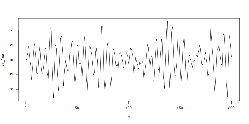
We can see a very distinct cyclic pattern where the process is very positively correlated with the previous value and very negatively correlated with the value before that. We can illustrate this by plotting a correlogram of a number of lagged values.

library(corrgram)
ar_four_lags <- data.frame(current = ar_four[-c(197, 198, 199, 200)],
                           lag1 = ar_four[-c(1, 198, 199, 200)],
                           lag2 = ar_four[-c(1, 2, 199, 200)],
                           lag3 = ar_four[-c(1, 2, 3, 200)],
                           lag4 = ar_four[-c(1, 2, 3, 4)])

corrgram(ar_four_lags)

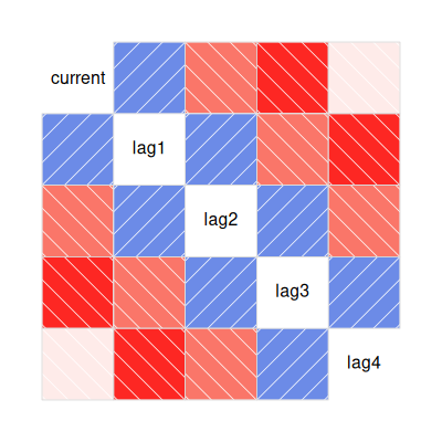
We see that adjacent values (e.g. current & lag1 or lag2 & lag3) are highly correlated, since $\beta_1 = 0.8$. The intuition here is that since the weight is quite high, the process gets pulled in the same direction as that lag. Similarly since $\beta_2 = -0.8$ there we can see negative correlation between lags that are two steps apart.

What may be surprising is the stronger negative correlation for values three time steps apart. Without loss of generality, recall that since we are using an $AR(2)$ model, the current value is constructed as a linear combination of lag1 and lag2, with positive weight on lag1 and a negative weight on lag2. But we can see that lag1 is negatively correlated with lag3 and lag2 is strongly positively correlated with lag3. Therefore we should indeed expect strong negative correlation with lag3.

We see weaker correlation between current and lag2 than lag1 since there’s two random disturbances as opposed to one. This also explains the dropping correlation between current and lag4.

Stationary and non-stationary processes

A stochastic process is said to be stationary when the joint distribution of a selection of time indices is time invariant. That is to say given a set of time indices $t_1 < t_2 < \ldots < t_m$, the joint distribution of $(S_{t_1}, S_{t_2}, \ldots, S_{t_m})$ is identical to $(S_{t_1 + h}, S_{t_2 + h}, \ldots, S_{t_m + h})$ for $h \in Z^+$. Simply, the distribution of values for the process does not change over time and is “stationary”. Alternatively a process which is not stationary is non-stationary.

This is a useful albeit strong property to have. It implies that modelling a subset of the process is sufficient to be able to use that model to extrapolate forward and make convincing forecasts of the process. The first step in modelling non-stationary is often to apply transformations to make it stationary (differencing, log, etc).

In practice we often work with the weaker property of weak stationarity. For a process to be weakly stationary it must have

A constant and finite mean (i.e. $\mathbb{E}[S_t] = μ, \, ∀ t $)
A finite second moment (i.e. $\mathbb{E}[|S_t^2|] < ∞, \, ∀ t $)
Time invariant autocorrelation (i.e. the correlation between lags is equal for all lags that are a particular number of time steps apart).

Auto-regressive processes are weakly stationary under some weak restrictions. In the examples about we chose very specific values for $\beta$. Picking random values may lead to a non-stationary process. In fact the first example, the random walk, is non-stationary since its variance is proportional to time (since $S_t$ is just the sum of $t$ normally distributed variables) and therefore unbounded.

For an $AR(1)$ model to be weakly stationary we require $|\beta_1| < 1$. For higher order processes the requirement is slightly more complicated. An $AR(n)$ model is stationary if all complex roots of the polynomial $\Phi(z) = 1 - \sum_{i=1}^n \beta_i z^i$ lie outside of the unit circle.

References

Wooldridge, Jeffrey M., 1960-. (2012). Introductory econometrics : a modern approach. Mason, Ohio :South-Western Cengage Learning